2018-09-17 (Last Updated: 2024-07-17)

Strange Attractors App#

Strange attractors are a type of iterative equation that traces the path of a particle through a 2D space, forming interesting patterns in the trajectories. The patterns differ depending on which sets of equations are used and which parameter values are selected for those equations.

To make the parameter spaces easy to explore, we’ll build a web-based application using Panel to select between the attractor families, adjust the parameter values for that type of attractor, and see the results rendered using Datashader. Using this app requires a live, running Python process, not just a static web page.

This dashboard code also functions as an example of how to build a Panel application for working with an arbitrarily large family of Python objects organized into a class hierarchy, without depending on the details of that structure and without that code depending on any GUI libraries. In this approach, each object defines its own parameters in a GUI-independent way, but then Panel can access this information and construct appropriate widgets to provide interactive control of the values. This approach can allow the same codebase be used in a GUI with full interactivity while also supporting non-GUI command-line, batch, or headless usage. New classes added to the .py file, even with entirely different parameters, will automatically be supported by this GUI code.

If you aren’t familiar with Panel, you may wish to check out the much simpler Clifford-only app first, to understand the basic structure of an app and of how to compute an attractor.

Attractor definitions#

Here, we’ll make use of a family of attractors whose code is defined in the separate file attractors.py, currently including classes for Clifford, De Jong, Svensson, Fractal Dream, Bedhead, Hopalong1, Hopalong2, Gumowski Mira, and Symmetric Icon attractors. That module also provides support for working with a separate YAML-format list of examples of each type of attractor, in attractors.yml.

Each attractor family is a subclass of the Attractor class, capturing the attractor equations as runnable Python code, the equations in LaTeX form for displaying, the parameters of the equations, and their expected ranges of values:

import attractors

h = attractors.Hopalong1()
h

Hopalong1(a=9.8, b=4.1, c=3.8, colormap='kgy', equations=['$x_{n+1} = y_n-\\mathrm{sgn}(x_n)\\sqrt{\\left|\\ bx_n-c\\ \\right|}$', '$y_{n+1} = a-x_n$'], name='Hopalong100002', x=0, y=0)

from IPython.display import display, Latex

display(*[Latex(e) for e in h.equations])

\[x_{n+1} = y_n-\mathrm{sgn}(x_n)\sqrt{\left|\ bx_n-c\ \right|}\]

\[y_{n+1} = a-x_n\]

import inspect

print(inspect.getsource(h.fn))

    @staticmethod
    @jit
    def fn(x, y, a, b, c, *o):
        return y - sqrt(fabs(b * x - c)) * np.sign(x), \
               a - x

We can use the trajectory function to run this equation for specified parameter values to calculate n (x,y) positions of the simulated particle through space, where each subsequent position is calculated from the previous one:

attractors.trajectory(h.fn, 0, 0, a=1, b=3, c=5, n=5)

	x	y
0	0.000000	0.000000
1	0.000000	1.000000
2	1.000000	1.000000
3	-0.414214	0.000000
4	2.498528	1.414214

Attractor parameter values#

Many of these attractors have only specific sets of parameters that are visually striking. Suitable parameters have been collected into a separate YAML-format text file, which we can load here, add new values to, save, etc.:

params = attractors.ParameterSets(name="Attractors")
params.attractors["Svensson"]

Svensson(a=1.4, b=1.56, c=1.4, colormap='fire', d=-6.56, equations=['$x_{n+1} = d\\ \\sin\\ ax_n - \\sin\\ by_n$', '$y_{n+1} = c\\ \\cos\\ ax_n + \\cos\\ by_n$'], name='Svensson parameters', x=0, y=0)

The params object also allows constructing a new Attractor object by name with the given parameters:

params.attractor('Gumowski_Mira', None, 0.1, 0.1, 0.0, 0.5, -0.75)

Gumowski_Mira(a=0.0, b=0.5, colormap=None, equations=['$G(x) = \\mu x + \\frac{2(1-\\mu)x^2}{1+x^2}$', '$x_{n+1} = y_n + ay_n(1-by_n^2) + G(x_n)$', '$y_{n+1} = -x_n + G(x_{n+1})$'], mu=-0.75, name='Gumowski_Mira parameters', x=0.1, y=0.1)

Attractor plotting using Datashader#

To turn the attractors into visible images, we’ll define some plotting code using Datashader:

import datashader as ds
from datashader.colors import inferno, viridis
from colorcet import palette

palette["viridis"] = viridis
palette["inferno"] = inferno
size = 1000

def datashade(df, plot_type='points', cmap=palette["inferno"], size=size):
    cvs = ds.Canvas(plot_width=size, plot_height=size)
    agg = getattr(cvs,plot_type)(df, 'x', 'y', agg=ds.count())
    return ds.tf.shade(agg, cmap=cmap)

datashade(attractors.trajectory(attractors.Hopalong1.fn, 0, 0, a=1, b=3, c=5, n=5000000), cmap=viridis, size=200)

/home/runner/work/examples/examples/attractors/envs/default/lib/python3.11/site-packages/dask/dataframe/__init__.py:31: FutureWarning: 
Dask dataframe query planning is disabled because dask-expr is not installed.

You can install it with `pip install dask[dataframe]` or `conda install dask`.
This will raise in a future version.

  warnings.warn(msg, FutureWarning)

Panel dashboard#

As illustrated above, we can use datashade on its own to plot any of these attractors, or IPython.display.Latex to render the equations mathematically. But to make it much simpler to explore, let’s build an app with widgets using Panel. We’ll first make an object that lets us select between attractor families, types of plots, etc.:

import param, panel as pn
from panel.pane import LaTeX
pn.extension('katex', sizing_mode='stretch_width')

pn.Param.margin = 0
pn.widgets.Button.param.width.default = 300

class Attractors(pn.viewable.Viewer):
    attractor_type = param.Selector(objects=params.attractors, default=params.attractors["Clifford"], precedence=0.9)

    parameters = param.Selector(objects=params.attractors, precedence=-0.5, readonly=True)

    plot_type = param.Selector(
        precedence=0.8, objects=['points', 'line'],
        doc="Type of aggregation to use"
    )

    n = param.Integer(2000000, bounds=(1,None), softbounds=(1,50000000),
                      doc="Number of points", precedence=0.85)

    @param.depends("parameters.param", watch=True)
    def _update_from_parameters(self):
        a = params.attractor(*self.attractor_type())
        if a is not self.attractor_type:
            self.param.update(attractor_type=a)

    @param.depends("attractor_type.param", "plot_type", "n")
    def __panel__(self):
        return datashade(self.attractor_type(n=self.n), self.plot_type,
                         palette[self.attractor_type.colormap][::-1])

    @param.depends("attractor_type")
    def equations(self):
        if not self.attractor_type.equations:
            return pn.Column()
        return pn.Column("<b>"+self.attractor_type.__class__.name+" attractor<b>",
                         *[LaTeX(e) for e in self.attractor_type.equations])

ats = Attractors(name="Options")
params.current = lambda: ats.attractor_type
ats # Uncomment to see a plot of the current attractor

And we’ll create a scrubber widget to make it easy to select between the existing example parameter sets:

from panel.widgets import DiscretePlayer

player = DiscretePlayer(options=params.param.example.objects, interval=2000, align='center')
player.link(params, value='example');

And let’s add the panel logo and define some explanatory text that will be useful if this app is deployed outside the notebook context where you are reading this:

logo = '<img src="https://panel.holoviz.org/_static/logo_stacked.png" width=180 height=151>'
text = """ *This [Panel](https://github.com/holoviz/panel) app lets you explore [strange attractors](attractors.ipynb) 
-- fractal-like patterns that can emerge from the trajectory of a particle in 2D space.*

*Here you can choose between different attractor families, selecting from predefined examples or 
adjusting your own values and adding them to the saved list when you discover something interesting.*

*The trajectories are calculated quickly using [Numba](https://numba.pydata.org), aggregated using [Datashader](https://datashader.org), 
and colorized using [Colorcet](https://colorcet.holoviz.org).*"""
plot = pn.Column(ats, player)
widgets = pn.Param(ats.param, expand=True, margin=0)

Ok, now we are ready to put everything together into a dashboard using one of the available panel templates, which we will mark .servable() to indicate that the dashboard should be displayed if this notebook is run using panel serve:

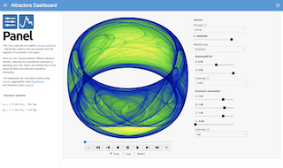
template = pn.template.FastGridTemplate(
    title="Strange Attractors Dashboard",
    sidebar=[logo, text, ats.equations],
    sidebar_width=250,
    accent="#4099da",
    theme_toggle=False
)

template.main[:6, 0:8] = plot
template.main[:6, 8:10] = widgets

template.servable();

You can add .show() after .servable() if you want to launch a standalone dashboard immediately from within the Jupyter notebook, or just run this notebook through Bokeh Server using panel serve --show attractors_panel.ipynb. Either way, you should get a browser tab with a dashboard like in the above cell, which you can explore or share.