Square Limit#
Square Limit#

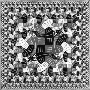
The above image shows a famous woodcut by M.C. Escher called Square Limit composed of tesselating fish tiles. In this notebook, we will recreate this pattern using the HoloViews Spline element.
The construction used here is that of Peter Henderson’s Functional Geometry paper and this notebook was inspired by Massimo Santini’s programming-with-escher notebook, itself inspired by Haskell and Julia implementations.
We start by importing HoloViews and NumPy and loading the extension:
import holoviews as hv
from holoviews import opts
import numpy as np
hv.extension('matplotlib')
This notebook makes extensive use of the Spline element and we will want to keep equal aspects and suppress the axes:
opts.defaults(opts.Spline(xaxis=None, yaxis=None, aspect='equal', bgcolor='white', linewidth=0.8))
‘Square Limit’ is composed from the following fish pattern, over which we show the unit square:
spline=[(0.0,1.0),(0.08,0.98),(0.22,0.82),(0.29,0.72),(0.29,0.72),(0.3,0.64),(0.29,0.57),(0.3,0.5),
(0.3,0.5),(0.34,0.4),(0.43,0.32),(0.5,0.26),(0.5,0.26),(0.58,0.21),(0.66,0.22),(0.76,0.2),(0.76,0.2),
(0.82,0.12),(0.94,0.05),(1.0,0.0),(1.0,0.0),(0.9,0.03),(0.81,0.04),(0.76,0.05),(0.76,0.05),(0.69,0.04),
(0.62,0.04),(0.55,0.04),(0.55,0.04),(0.49,0.1),(0.4,0.17),(0.35,0.2),(0.35,0.2),(0.29,0.24),(0.19,0.28),
(0.14,0.31),(0.14,0.31),(0.09,0.35),(-0.03,0.43),(-0.05,0.72),(-0.05,0.72),(-0.04,0.82),(-0.02,0.95),(0.0,1.0),
(0.1,0.85),(0.14,0.82),(0.18,0.78),(0.18,0.75),(0.18,0.75),(0.16,0.74),(0.14,0.73),(0.12,0.73),(0.12,0.73),
(0.11,0.77),(0.11,0.81),(0.1,0.85),(0.05,0.82),(0.1,0.8),(0.08,0.74),(0.09,0.7),(0.09,0.7),(0.07,0.68),
(0.06,0.66),(0.04,0.67),(0.04,0.67),(0.04,0.73),(0.04,0.81),(0.05,0.82),(0.11,0.7),(0.16,0.56),(0.24,0.39),
(0.3,0.34),(0.3,0.34),(0.41,0.22),(0.62,0.16),(0.8,0.08),(0.23,0.8),(0.35,0.8),(0.44,0.78),(0.5,0.75),
(0.5,0.75),(0.5,0.67),(0.5,0.59),(0.5,0.51),(0.5,0.51),(0.46,0.47),(0.42,0.43),(0.38,0.39),(0.29,0.71),
(0.36,0.74),(0.43,0.73),(0.48,0.69),(0.34,0.61),(0.38,0.66),(0.44,0.64),(0.48,0.63),(0.34,0.51),(0.38,0.56),
(0.41,0.58),(0.48,0.57),(0.45,0.42),(0.46,0.4),(0.47,0.39),(0.48,0.39),(0.42,0.39),(0.43,0.36),(0.46,0.32),
(0.48,0.33),(0.25,0.26),(0.17,0.17),(0.08,0.09),(0.0,0.01),(0.0,0.01),(-0.08,0.09),(-0.17,0.18),(-0.25,0.26),
(-0.25,0.26),(-0.2,0.37),(-0.11,0.47),(-0.03,0.57),(-0.17,0.26),(-0.13,0.34),(-0.08,0.4),(-0.01,0.44),
(-0.12,0.21),(-0.07,0.29),(-0.02,0.34),(0.05,0.4),(-0.06,0.14),(-0.03,0.23),(0.03,0.28),(0.1,0.34),(-0.02,0.08),
(0.02,0.16),(0.09,0.23),(0.16,0.3)]

unitsquare = hv.Bounds((0,0,1,1))
fish = hv.Spline((spline, [1,4,4,4]*34)) # Cubic splines
fish * unitsquare
As you may expect, we will be applying a number of different geometric transforms to generate ‘Square Limit’. To do this we will use Affine2D from matplotlib.transforms and matplotlib.path.Path (not to be confused with hv.Path!).
from matplotlib.path import Path
from matplotlib.transforms import Affine2D

# Define some Affine2D transforms
rotT = Affine2D().rotate_deg(90).translate(1, 0)
rot45T = Affine2D().rotate_deg(45).scale(1. / np.sqrt(2.), 1. / np.sqrt(2.)).translate(1 / 2., 1 / 2.)
flipT = Affine2D().scale(-1, 1).translate(1, 0)

def combine(obj):
    "Collapses overlays of Splines to allow transforms of compositions"
    if not isinstance(obj, hv.Overlay): return obj
    return hv.Spline((np.vstack([el.data[0] for el in obj.values()]),
                      np.hstack([el.data[1] for el in obj.values()])))

def T(spline, transform):
    "Apply a transform to a spline or overlay of splines"
    spline = combine(spline)
    result = Path(spline.data[0], codes=spline.data[1]).transformed(transform)
    return hv.Spline((result.vertices, result.codes))

# Some simple transform functions we will be using
def rot(el):        return T(el,rotT)
def rot45(el):      return T(el, rot45T)
def flip(el):       return T(el, flipT)
Here we define three Affine2D transforms (rotT,rot45T and flipT), a function to collapse HoloViews Spline overlays (built with the * operator) in a single Spline element, a generic transform function T and the three convenience functions we will be using directly (rot, rot45 and flip). Respectively, these functions rotate the spline by \(90^o\), rotate the spline by \(45^o\) and flip the spline horizontally.
Here is a simple example of a possible tesselation:
fish * rot(rot(fish))
Next we need two functions, beside and above to place splines next to each other or one above the other, while compressing appropriately along the relevant axis:
def beside(spline1, spline2, n=1, m=1):
    den = n + m
    t1 = Affine2D().scale(n / den, 1)
    t2 = Affine2D().scale(m / den, 1).translate(n / den, 0)
    return combine(T(spline1, t1) * T(spline2, t2))

def above(spline1, spline2, n=1, m=1):
    den = n + m
    t1 = Affine2D().scale(1, n / den).translate(0, m / den)
    t2 = Affine2D().scale(1, m / den)
    return combine(T(spline1, t1) * T(spline2, t2))

beside(fish, fish)* unitsquare + above(fish,fish) * unitsquare
One import tile in ‘Square Limit’ is what we will call smallfish which is our fish rotate by \(45^o\) then flipped:
smallfish = flip(rot45(fish))
smallfish * unitsquare
We can now build the two central tesselations that are necessary to build ‘Square Limit’ which we will call t and u respectively:
t =  fish *  smallfish * rot(rot(rot(smallfish)))
u = smallfish * rot(smallfish) * rot(rot(smallfish)) * rot(rot(rot(smallfish)))
t *unitsquare + u * unitsquare
We are now ready to define the two recursive functions that build the sides and corners of ‘Square Limit’ respectively. These recursive functions make use of quartet which is used to compress four splines into a small 2x2 grid:
blank = hv.Spline(([(np.nan, np.nan)],[1])) # An empty Spline object useful for recursion

def quartet(p, q, r, s):
    return above(beside(p, q), beside(r, s))

def side(n):
    if n == 0:
        return hv.Spline(([(np.nan, np.nan)],[1]))
    else:
        return quartet(side(n-1), side(n-1), rot(t), t)

def corner(n):
    if n == 0:
        return hv.Spline(([(np.nan, np.nan)],[1]))
    else:
        return quartet(corner(n-1), side(n-1), rot(side(n-1)), u)


corner(2) + side(2)
We now have a way of building the corners and sides of ‘Square Limit’. To do so, we will need one last function that will let us put the four corners and four sides in place together with the central tile:
def nonet(p, q, r, s, t, u, v, w, x):
    return above(beside(p, beside(q, r), 1, 2),
                 above(beside(s, beside(t, u), 1, 2),
                       beside(v, beside(w, x), 1, 2)), 1, 2)

args = [fish]* 4 + [blank] + [fish] * 4
nonet(*args)
Here we see use nonet to place eight of our fish around the edge of the square with a blank in the middle. We can finally use nonet together with our recursive corner and side functions to recreate ‘Square Limit’:
def squarelimit(n):
    return nonet(corner(n), side(n), rot(rot(rot(corner(n)))),
                 rot(side(n)), u, rot(rot(rot(side(n)))),
                 rot(corner(n)), rot(rot(side(n))), rot(rot(corner(n))))
hv.output(squarelimit(3), size=250)