2018 FIFA World Cup#

The FIFA World Cup is the premier international football tournament, held every four years and featuring teams from around the globe. It is a celebration of the sport, bringing together fans and players in a thrilling competition for the prestigious title. Each World Cup tournament offers a wealth of data on matches, players, and events, providing a rich resource for analysis and visualization.
In this notebook, we focus on the 2018 FIFA World Cup, hosted by Russia. Using hvPlot and Panel, we will create dynamic and interactive visualizations to explore the extensive dataset from this tournament. These tools enable us to investigate the statistics and uncover insights about player performances and more.
The dataset used for this analysis is sourced from Pappalardo, Luca; Massucco, Emanuele (2019) Soccer match event dataset, figshare collection.
Load the data#
Here we will load the players and World Cup events dataset from the figshare collection to enable us create plots and visualizations focused only on the 2018 World Cup.
import numpy as np
import pandas as pd
import hvplot.pandas # noqa
import holoviews as hv
from holoviews import opts
import panel as pn

pn.extension(sizing_mode='stretch_width')
players_df = pd.read_json('data/players.json', encoding='unicode-escape')
events_df = pd.read_json('data/events/events_World_Cup.json')
events_df.head(2)
| eventId | subEventName | tags | playerId | positions | matchId | eventName | teamId | matchPeriod | eventSec | subEventId | id | |
|---|---|---|---|---|---|---|---|---|---|---|---|---|
| 0 | 8 | Simple pass | [{'id': 1801}] | 122671 | [{'y': 50, 'x': 50}, {'y': 53, 'x': 35}] | 2057954 | Pass | 16521 | 1H | 1.656214 | 85 | 258612104 |
| 1 | 8 | High pass | [{'id': 1801}] | 139393 | [{'y': 53, 'x': 35}, {'y': 19, 'x': 75}] | 2057954 | Pass | 16521 | 1H | 4.487814 | 83 | 258612106 |
players_df.tail(2)
| passportArea | weight | firstName | middleName | lastName | currentTeamId | birthDate | height | role | birthArea | wyId | foot | shortName | currentNationalTeamId | |
|---|---|---|---|---|---|---|---|---|---|---|---|---|---|---|
| 3601 | {'name': 'Morocco', 'id': 504, 'alpha3code': '... | 70 | Ahmed Reda | Tagnaouti | 16183 | 1996-04-05 | 182 | {'code2': 'GK', 'code3': 'GKP', 'name': 'Goalk... | {'name': 'Morocco', 'id': 504, 'alpha3code': '... | 285583 | right | A. Tagnaouti | null | |
| 3602 | {'name': 'Panama', 'id': 591, 'alpha3code': 'P... | 0 | Ricardo | Guardia Avila | 62943 | 1997-02-04 | 0 | {'code2': 'MD', 'code3': 'MID', 'name': 'Midfi... | {'name': 'Panama', 'id': 591, 'alpha3code': 'P... | 361536 | left | R. Avila | null |
Plots#
Event distribution#
We can take a look at the unique events that take place in a typical football game and plot the frequency of those events using a hvPlot bar chart:
event_type_count = events_df['eventName'].value_counts()
event_type_distribution = event_type_count.hvplot.bar(
    title='Distribution of Event Types', height=400,
    responsive=True, rot=45,
)
event_type_distribution
It is unsurprising that passes are the most common event in a football match, however we would also like to see the areas of the football pitch where most of these events occur.
First, we will use the HoloViews library to draw an outline of a football pitch using the official dimensions:
opts.defaults(opts.Path(color='black'),
              opts.Rectangles(color=''),
              opts.Points(color='black', size=5))
# Set the dimensions of the field in meters
field_length = 105
field_width = 68
penalty_area_length = 16.5
penalty_area_width = 40.3
goal_area_length = 5.5
goal_area_width = 18.32
goal_width = 7.32
goal_depth = 2.44

pitch_plot_height = 550
pitch_plot_width = 800

# Helper function to create arcs
def create_arc(center, radius, start_angle, end_angle, clockwise=False):
    if clockwise:
        angles = np.linspace(np.radians(start_angle), np.radians(end_angle), 100)
    else:
        if start_angle < end_angle:
            start_angle += 360
        angles = np.linspace(np.radians(start_angle), np.radians(end_angle), 100)
    x = center[0] + radius * np.cos(angles)
    y = center[1] + radius * np.sin(angles)
    return hv.Path([np.column_stack([x, y])])

# create football pitch
def plot_pitch():
    pitch_elements = [
        hv.Rectangles([(0, 0, field_length, field_width)]), # outer pitch rectangle
        hv.Ellipse(field_length/2, field_width/2, 18.3), # center circle
        hv.Points([(field_length/2, field_width/2)]), # center spot
        hv.Path([[(field_length/2, 0), (field_length/2, field_width)]]), # halfway line
        hv.Rectangles([(0, (field_width - penalty_area_width) / 2, penalty_area_length,
                        (field_width + penalty_area_width) / 2)]), # left penalty area
        hv.Rectangles([(field_length - penalty_area_length, (field_width - penalty_area_width) / 2,
                        field_length, (field_width + penalty_area_width) / 2)]), # right penalty area
        hv.Rectangles([(0, (field_width - goal_area_width) / 2, goal_area_length,
                        (field_width + goal_area_width) / 2)]), # left goal area
        hv.Rectangles([(field_length - goal_area_length, (field_width - goal_area_width) / 2,
                        field_length, (field_width + goal_area_width) / 2)]), # right goal area
        hv.Points([(11, field_width/2)]), # left penalty spot
        hv.Points([(field_length - 11, field_width/2)]), # right penalty spot
        create_arc((11, field_width/2), 9.15, 52, 308), # left penalty arc
        create_arc((field_length - 11, field_width/2), 9.15, 232, 128), # right penalty arc
        hv.Rectangles([(-goal_depth, (field_width - goal_width) / 2,
                        0, (field_width + goal_width) / 2)]), # left goal
        hv.Rectangles([(field_length, (field_width - goal_width) / 2,
                        field_length + goal_depth, (field_width + goal_width) / 2)]), # right goal
        hv.Arrow(20, 5, '', '>', ), # attack arrow
        hv.Text(10, 6, 'Attack', 11) # attack text
    ]

    field = hv.Overlay(pitch_elements).opts(
        frame_width=pitch_plot_width, frame_height=pitch_plot_height,
        xlim=(-5, field_length + 5), ylim=(-5, field_width + 5),
        xaxis=None, yaxis=None
    )
    return field
pitch = plot_pitch()
pitch
In events_df dataframe, the positions column is a pair of coordinates written in percentages instead of the actual field dimensions, as described in the data source. To match the coordinates of the drawn pitch, we will have to transform those coordinates to their actual dimensions in meters:
def transform_positions(events_df, field_length, field_width):
    def scale_position(pos):
        scaled_positions = []
        for p in pos:
            scaled_p = {
                'x': p['x'] * field_length / 100,
                'y': p['y'] * field_width / 100
            }
            scaled_positions.append(scaled_p)
        return scaled_positions

    events_df['positions'] = events_df['positions'].apply(scale_position)
    return events_df
events_df = transform_positions(events_df, field_length, field_width)
events_df.head(2)
| eventId | subEventName | tags | playerId | positions | matchId | eventName | teamId | matchPeriod | eventSec | subEventId | id | |
|---|---|---|---|---|---|---|---|---|---|---|---|---|
| 0 | 8 | Simple pass | [{'id': 1801}] | 122671 | [{'x': 52.5, 'y': 34.0}, {'x': 36.75, 'y': 36.... | 2057954 | Pass | 16521 | 1H | 1.656214 | 85 | 258612104 |
| 1 | 8 | High pass | [{'id': 1801}] | 139393 | [{'x': 36.75, 'y': 36.04}, {'x': 78.75, 'y': 1... | 2057954 | Pass | 16521 | 1H | 4.487814 | 83 | 258612106 |
Then, we can generate a heatmap to see where these events occur the most on the pitch:
def plot_event_heatmap(events_df, event_type, cmap='Greens'):
    """
    Plots a heatmap of the specified event type on a football pitch.

    Parameters:
    events_df (pd.DataFrame): The dataframe containing event data with the following columns:
        - eventId: The identifier of the event's type.
        - eventName: The name of the event's type.
        - subEventId: The identifier of the subevent's type.
        - subEventName: The name of the subevent's type.
        - tags: A list of event tags describing additional information about the event.
        - eventSec: The time when the event occurs (in seconds since the beginning of the current half).
        - id: A unique identifier of the event.
        - matchId: The identifier of the match the event refers to.
        - matchPeriod: The period of the match (1H, 2H, E1, E2, P).
        - playerId: The identifier of the player who generated the event.
        - positions: The origin and destination positions associated with the event.
        - teamId: The identifier of the player's team.
    event_type (str): The type of event to plot from the eventName column.
    cmap (str): The color map to use for the heatmap. Default is 'Greens'.

    Returns:
    hvPlot object: A heatmap plot of the specified event type overlaid on a football pitch.
    """
    event_type = event_type.lower()
    event = events_df[events_df['eventName'].str.lower() == event_type]
    positions = [(pos[0]['x'], pos[0]['y']) for pos in event['positions'] if len(pos) > 0]
    event_df = pd.DataFrame(positions, columns=['x', 'y'])
    pitch = plot_pitch()
    title = f"{event_type.capitalize()} Heatmap for All Players"

    event_heatmap = event_df.hvplot.hexbin(x='x', y='y', cmap=cmap, min_count=1, title=title)

    event_heatmap_plot = (event_heatmap * pitch).opts(
        frame_width=pitch_plot_width, frame_height=pitch_plot_height,
        xlim=(-5, 110), ylim=(-5, 73), xaxis=None, yaxis=None
    )

    return event_heatmap_plot
For example, let use see the heatmap of the passes in a typical game:
passes_map = plot_event_heatmap(events_df, 'pass')
passes_map
We can replace “pass” with another event type to see the heatmap for that event. However, Panel makes it easy to create widgets that we can use to select the different event types and immediately see the heatmap of that event.
First, we create a Select widget and use pn.bind to link the widget with the event_heatmap function. Then we can display it as a column using pn.Column:
event_type = list(events_df['eventName'].unique())
event_type_selector = pn.widgets.Select(name='Event Type', options=event_type)
event_heatmap = pn.bind(plot_event_heatmap, events_df=events_df, event_type=event_type_selector)

pn.Column(event_type_selector, event_heatmap)
If you have a live python process running, you can use the Selector widget to alternate between the different event types and see their heatmap on the football pitch.
Player events#
Using the playerId from the events dataframe, we can plot the top n players in any event category. First, we create a function to find the top players for any event type:
def find_top_players(events_df, players_df, event_type, top_n=10):
    """
    Finds the top players for a given event type.

    Parameters:
    events_df (pd.DataFrame): The dataframe containing event data.
    players_df (pd.DataFrame): The dataframe containing player data.
    event_type (str): The type of event to filter by.
    top_n (int): The number of top players to return.

    Returns:
    pd.DataFrame: A dataframe containing the top players for the given event type.
    """
    event_type = event_type.lower()
    event = events_df[events_df['eventName'].str.lower() == event_type]
    event_counts = event.groupby('playerId').size().reset_index(name=f'{event_type} count')

    top_players = event_counts.sort_values(by=f'{event_type} count', ascending=False).head(top_n)
    top_players = top_players.merge(players_df, left_on='playerId', right_on='wyId')
    top_players.set_index('playerId', inplace=True)

    return top_players[['shortName', f'{event_type} count']]
For example, we can check the top 10 players with the most passes in the World Cup:
pass_maestros = find_top_players(events_df, players_df, 'pass')
pass_maestros
| shortName | pass count | |
|---|---|---|
| playerId | ||
| 3306 | Sergio Ramos | 482 |
| 9380 | J. Stones | 470 |
| 8287 | L. Modrić | 461 |
| 3563 | Isco | 447 |
| 36 | T. Alderweireld | 442 |
| 3476 | I. Rakitić | 404 |
| 8653 | H. Maguire | 398 |
| 3269 | Jordi Alba | 376 |
| 8277 | K. Walker | 370 |
| 31528 | N. Kanté | 360 |
We can then create a bar chart to visualize these players:
def plot_top_players(events_df, players_df, event_type, top_n=10):
    """
    Plots a bar chart of the top players for a given event type.

    Parameters:
    events_df (pd.DataFrame): The dataframe containing event data.
    players_df (pd.DataFrame): The dataframe containing player data.
    event_type (str): The type of event to filter by.
    top_n (int): The number of top players to return.

    Returns:
    hvPlot: A bar chart of the top players for the given event type.
    """
    top_players = find_top_players(events_df, players_df, event_type, top_n)
    event_type = event_type.lower()

    title = f'Top {top_n} Players for {event_type.capitalize()}'

    bar_plot = top_players.hvplot.bar(
        title=title, x='shortName', y=f'{event_type} count',
        xlabel='', ylabel=f'Number of {event_type}', rot=45, color='#177F3B'
    )

    return bar_plot
pass_maestros_plot = plot_top_players(events_df, players_df, 'pass')
pass_maestros_plot
Using Panel, we can also create another type of widget to select number of bars to display in the bar chart as well as selecting the different event types:
top_n_selector = pn.widgets.IntSlider(name='Top', start=1, end=20, value=10)

bar_chart = pn.bind(plot_top_players, events_df=events_df, players_df=players_df,
                    event_type=event_type_selector, top_n=top_n_selector)

pn.Column(pn.Row(top_n_selector, event_type_selector), bar_chart)
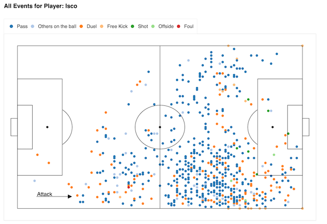
We can also plot the individual player activity for any type of event on the football pitch. First, we create a function that maps the player name to their unique ID, then create another function that plots the player activity using the resulting player ID:
def get_player_id(player_name):
    player_name_to_id = dict(zip(players_df['shortName'], players_df['wyId']))
    return player_name_to_id.get(player_name)

def plot_player_events(events_df, players_df, player_name):
    """
    Plots a distribution of events performed by a specific player on a football pitch.

    Parameters:
    events_df (pd.DataFrame): The dataframe containing event data.
    players_df (pd.DataFrame): The dataframe containing player data.
    player_name (str): The name of the player to plot events for.

    Returns:
    hvPlot object: A scatter plot of the player's events overlaid on a football pitch.
    """
    pitch = plot_pitch()
    if not player_name:
        return pn.Column(pn.pane.Markdown("## Start typing a player name above."), pitch)

    player_id = get_player_id(player_name)
    if player_id is None:
        return pn.Column(pn.pane.Markdown("## Please select a valid player."), pitch)

    player_events = events_df[events_df['playerId'] == player_id]

    if player_events.empty:
        return pn.Column(pn.pane.Markdown(f"## No events found for {player_name}."), pitch)

    positions = [(pos[0]['x'], pos[0]['y'], event)
                 for pos, event in zip(player_events['positions'], player_events['eventName'])
                 if len(pos) > 0]
    event_df = pd.DataFrame(positions, columns=['x', 'y', 'eventName'])

    event_scatter = event_df.hvplot.points(x='x', y='y', c='eventName', cmap='Category20',
                                           title=f'All Events for Player: {player_name}')

    player_scatter = (event_scatter * pitch).opts(frame_width=pitch_plot_width, frame_height=pitch_plot_height,
                                                  xlim=(-5, 110), ylim=(-5, 73),
                                                  xaxis=None, yaxis=None, legend_position='top')

    return player_scatter
isco_map = plot_player_events(events_df, players_df, 'Isco')
isco_map
Using the Panel AutocompleteInput widget, we can then devise a way to search for players using their names and immediately see their activities on the football pitch:
player_name_selector = pn.widgets.AutocompleteInput(
    name='Player Name', options=list(players_df['shortName']),
    placeholder='Type player name...', case_sensitive=False,
    search_strategy='includes', value='L. Messi'
)

player_events = pn.bind(plot_player_events, events_df=events_df,
                        players_df=players_df, player_name=player_name_selector)

pn.Column(player_name_selector, player_events)
Another insightful view would be to show the scatter plot of pass start locations for a selected player and then adding a callback function that shows the trajectory of the passes from a clicked location:
def plot_player_pass_trajectory(events_df, players_df, player_name):
    player_id = get_player_id(player_name)
    pitch = plot_pitch()

    if player_id is None:
        return pn.Column(pn.pane.Markdown("## Please select a valid player."), pitch)

    player_events = events_df[events_df['playerId'] == player_id]

    if player_events.empty:
        return pn.Column(pn.pane.Markdown(f"## No events found for {player_name}."), pitch)

    passes = player_events[player_events['eventName'].str.lower() == 'pass']

    if passes.empty:
        return pn.Column(pn.pane.Markdown(f"## No passes found for {player_name}."), pitch)

    pass_positions = [(pos[0]['x'], pos[0]['y']) for pos in passes['positions'] if len(pos) > 1]
    pass_df = pd.DataFrame(pass_positions, columns=['x', 'y'])

    pass_scatter = pass_df.hvplot.points(
        x='x', y='y', color='#1D78B4',
        title=f"Click for Pass Trajectories of {player_name}"
    )
    total_passes = hv.Text(75, 70, f'Total number of passes: {len(pass_df)}', halign='center', fontsize=12)

    # Callback to filter passes based on click location
    def filter_passes(x, y, radius=1.5):
        filtered_passes = passes[
            (passes['positions'].apply(lambda pos: pos[0]['x']) >= x - radius) &
            (passes['positions'].apply(lambda pos: pos[0]['x']) <= x + radius) &
            (passes['positions'].apply(lambda pos: pos[0]['y']) >= y - radius) &
            (passes['positions'].apply(lambda pos: pos[0]['y']) <= y + radius)
        ]

        if filtered_passes.empty:
            return hv.Overlay()

        pass_lines = []
        for pos in filtered_passes['positions']:
            pass_lines.append(hv.Segments([(pos[0]['x'], pos[0]['y'], pos[1]['x'], pos[1]['y'])]).opts(
                color='green', line_width=2, line_alpha=.5))
        pass_lines_overlay = hv.Overlay(pass_lines)

        return pass_lines_overlay

    # Create a stream for handling clicks
    stream = hv.streams.Tap(source=pass_scatter, x=52, y=34)
    dynamic_pass_lines = hv.DynamicMap(lambda x, y: filter_passes(x, y), streams=[stream])

    dynamic_map = pitch * pass_scatter * total_passes * dynamic_pass_lines

    return dynamic_map.opts(frame_width=pitch_plot_width, frame_height=pitch_plot_height,
                            xlim=(-5, 110), ylim=(-5, 73),
                            xaxis=None, yaxis=None)
Then we use the previously defined player_name_selector widget to bind it to the plot_player_pass_trajectory in other to make it easier to search for different players and view their passing:
player_pass_scatter = pn.bind(plot_player_pass_trajectory, events_df=events_df,
                         players_df=players_df, player_name=player_name_selector)

pn.Column(player_name_selector, player_pass_scatter, sizing_mode='stretch_width')
Clicking in the vicinity of any of these points will show the trajectory of the passes.
Dashboard#
We can now combine all the different plots into one layout using pn.Column with the widgets at the top:
all_players_tab = pn.Column(
    pn.Row(event_type_selector, top_n_selector),
    bar_chart,
    event_heatmap,
    sizing_mode='stretch_both',
)

player_event_tab = pn.Column(
    player_name_selector,
    player_events,
    player_pass_scatter,
    sizing_mode='stretch_both',
)

layout = pn.Tabs(('All Players', all_players_tab), ('Per Player', player_event_tab))
layout
Servable dashboard#
Now that we have a fully interactive dashboard, we can now deploy it in a template to give it a more polished look:
logo = '<img src="https://upload.wikimedia.org/wikipedia/en/6/67/2018_FIFA_World_Cup.svg" style="display: block; margin: 0 auto;">'

text = """ Explore the 2018 FIFA World Cup with interactive visualizations built with `hvPlot` and `Panel` from [HoloViz](https://holoviz.org/)."""

template = pn.template.FastListTemplate(
    header_background= '#177F3B',
    title='2018 FIFA World Cup Dashboard',
    sidebar=[logo, text],
    main=[layout],
    main_layout=None,
    main_max_width="800px",
)
template.servable();
You can now display this as a standalone app from the command line using panel serve world_cup.ipynb --show