Time-Lapse Microscopy#

hvplotpanelholoviewsbokehdatashaderholonotexarraydask

Published: November 21, 2024 · Modified: December 4, 2024

Open app(s) Run notebook Download project

Time-Lapse Microscopy header

Overview#

This workflow demonstrates the display of time-lapse microscopy in neuroscience. Each frame in the image-stack dataset corresponds to a concurrent time sample, typically intended to capture a dynamic process of living cells.

For example, a dynamic process of interest could be neural action potentials, and the data might come from a miniature microscope (see image in this notebook’s header) that captures the change in fluorescence of special proteins caused by electrochemical fluctuations indicative of neuronal activity. These video-like datasets often contain many more frames in the ‘Time’ dimension compared to the number of pixels in the height or width of each frame.

App Versions#

We will build three different visualization approaches to cater to different use cases:

Basic Viewer: A one-line application using hvPlot, a high-level package that wraps HoloViews. This version is ideal for quick inspections and preliminary analyses of image stacks.
Intermediate Viewer with Side Views: Uses HoloViews for additional interactive elements, scalebars, and linked side views, aiding better navigation of the image stack and identification of regions of interest.
Advanced Viewer with Annotations and Linked Timeseries: Building from the intermediate HoloViews viewer, this version adds annotation capabilities using HoloNote, allowing for interactive spatial annotations with linked timeseries.

These applications are designed to handle large datasets efficiently, leveraging tools like Xarray, Dask, and Zarr for scalable data management.

Prerequisites#

Topic	Type	Notes
Xarray Tutorial	Prerequisite	Essential introduction to working with `xarray` data

Imports and Configuration#

from pathlib import Path
import numpy as np
import pandas as pd
import xarray as xr
import holoviews as hv
from holoviews.operation.datashader import rasterize
import hvplot.xarray # noqa
import panel as pn
import fsspec

pn.extension('tabulator')
hv.extension('bokeh')

Loading and Inspecting the Data#

We’ll be working with a sample dataset of time-lapse microscopy images. The dataset is stored in Zarr format, which is optimized for chunked, compressed, and scalable storage.

DATA_URL = 'https://datasets.holoviz.org/miniscope/v1/real_miniscope_uint8.zarr/'
DATA_DIR = Path('./data')
DATA_FILENAME = Path(DATA_URL).name
DATA_PATH = DATA_DIR / DATA_FILENAME

print(f'Local Data Path: {DATA_PATH}')

Local Data Path: data/real_miniscope_uint8.zarr

Let’s download the dataset (if it wasn’t already) so we can have a local copy and avoid any network delays. However, this workflow should also work if the dataset stays remote (thanks to Xarray, Zarr, Dask, and other scalability-providing tools), such as when it’s too large to reasonably download in its entirety.

Note

If you are viewing this notebook as a result of using the `anaconda-project run` command, the data has already been ingested, as configured in the associated yaml file. Running the following cell should find that data and skip any further download.

Warning

If the data was not previously ingested with `anaconda-project`, the following cell will download ~300 MB the first time it is run.

DATA_DIR.mkdir(parents=True, exist_ok=True)

# Download the data if it doesn't exist
if not DATA_PATH.exists():
    print(f'Downloading data to: {DATA_PATH}')
    ds_remote = xr.open_dataset(
        fsspec.get_mapper(DATA_URL), engine='zarr', chunks={}
    )
    ds_remote.to_zarr(str(DATA_PATH))  # Save locally
    print(f'Dataset downloaded to: {DATA_PATH}')
else:
    print(f'Data exists at: {DATA_PATH}')

Data exists at: data/real_miniscope_uint8.zarr

Now, let’s load the dataset using xarray, specifying chunks for efficient data handling with Dask.

# Open the dataset from the local copy
ds = xr.open_dataset(
    DATA_PATH,
    engine='zarr',
    chunks={'frame': 400, 'height': -1, 'width': -1}  # Chunk by frames
)

# Access the variable 'varr_ref' which contains the image data
da = ds['varr_ref']
da

<xarray.DataArray 'varr_ref' (frame: 2000, height: 480, width: 752)> Size: 722MB
dask.array<open_dataset-varr_ref, shape=(2000, 480, 752), dtype=uint8, chunksize=(400, 480, 752), chunktype=numpy.ndarray>
Coordinates:
  * frame    (frame) int64 16kB 0 1 2 3 4 5 6 ... 1994 1995 1996 1997 1998 1999
  * height   (height) int64 4kB 0 1 2 3 4 5 6 7 ... 473 474 475 476 477 478 479
  * width    (width) int64 6kB 0 1 2 3 4 5 6 7 ... 745 746 747 748 749 750 751

The dataset da is a 3D array with dimensions (frame, height, width). Each frame corresponds to a time point in the image stack.

App V1: Basic Viewer with hvPlot#

Our first application is a simple viewer using hvPlot, which allows for quick visualization of the image stack with minimal code.

hvplot_app = da.hvplot.image(
    groupby="frame",
    title='hvPlot App',
    cmap='viridis',
    clim=(0, 20),
    data_aspect=1,
    widget_location='bottom',
)
# hvplot_app

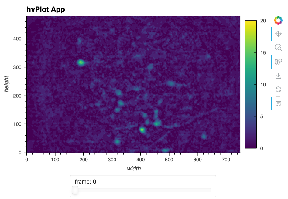
Here’s a static snapshot of what the previous cell produces in a live notebook - the quick hvPlot app. 👉

To facilitate widget-interactivity on static websites, we can embed the data right in the HTML output by using dynamic=False. But we’ll only do this on a subset of the frames to avoid overloading every visitor to the site:

da_subset = da.isel(frame=slice(20, 40))

da_subset.hvplot.image(
    dynamic=False,  # Embeds all frames in webpage. Only do this with a few frames.
    groupby="frame",
    title='Use my widget on a static website!',
    cmap='viridis',
    clim=(0, 20),
    data_aspect=1,
    widget_location='bottom',
)

As you can see, this creates an interactive image viewer where you can navigate through frames using a slider widget. Not much more needs to be said about that; it’s simple and effective in a pinch!

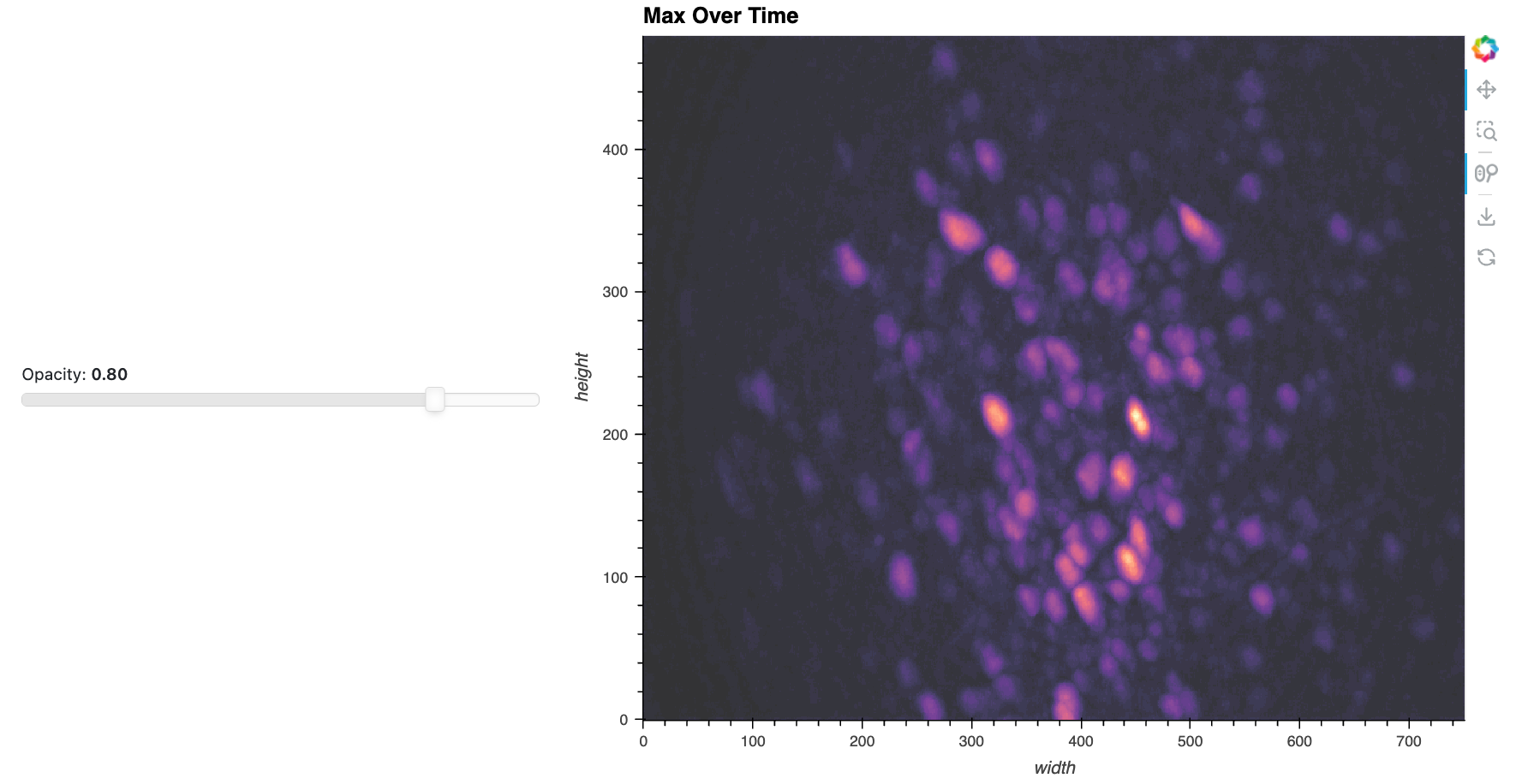
To easily enrich and extend this simple app, we do things like add a maximum-projection image so we can see the maximum fluorescence per pixel and visually locate the potential neurons in two-dimensions.

max_proj = da.max('frame').compute().astype(np.float32)
img_max_proj = max_proj.hvplot.image(
    title='Max Over Time',
    cmap="magma",
    clim=(0,20),
    data_aspect=1,
)
img_max_proj

Note

Displaying the same interactive views or components across different cells in a notebook may lead to unintended consequences, as they are intentionally linked by default and can interfere. For this reason, many of the previews of the incremental steps in this tutorial are static previews.

# pn.Row(hvplot_app, img_max_proj)

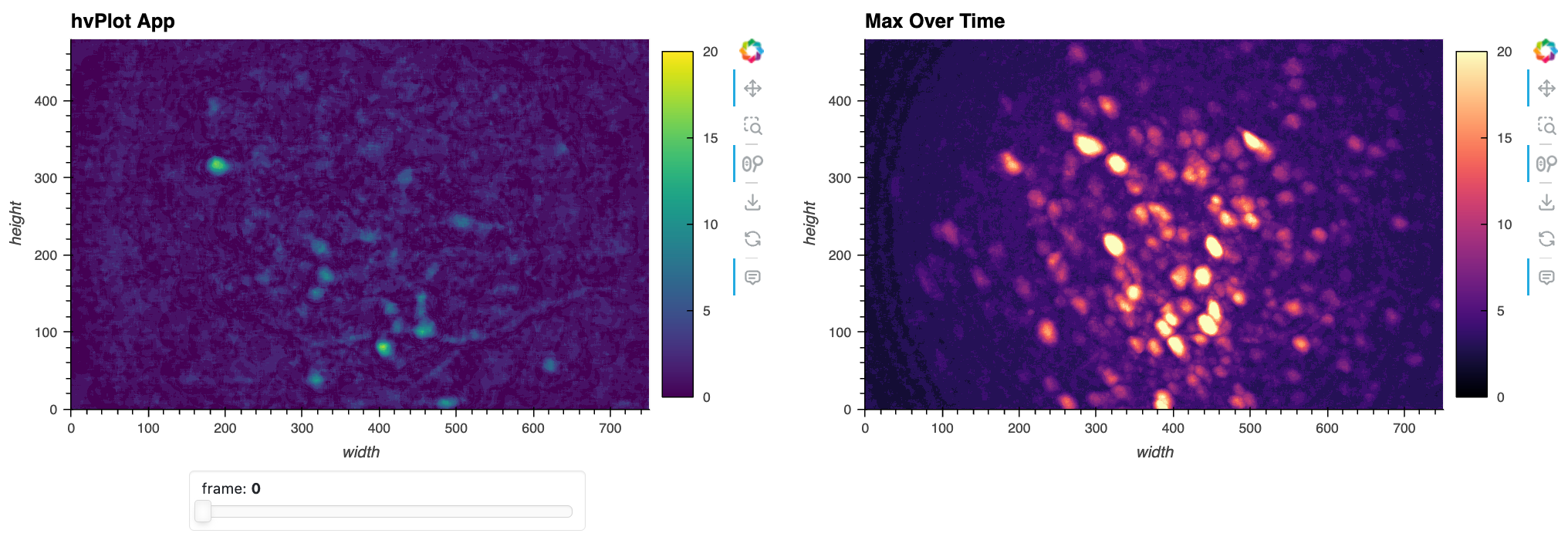
Here’s a static snapshot of what the previous cell produces - the basic app with a max projection over time. 👉

This was a quick way to see one frame at a time! But it looks like there are a lot of fluorescent blobs (candidate neurons) in the ‘Max Over Time’ image and now we want a quick way to visually locate and navigate to the relevant frames in the image stack.

App V2: Intermediate Viewer with Side Views#

While we could continue usinghvPlot to extend our basic app, we’ll switch to the slightly lower-level HoloViews (the library underlying hvPlot) for greater control as we handle the added complexity of our three-dimensional data array. To build a more advanced application, we’ll pair HoloViews with Panel for enhanced layout customization and interactive linking.

This more advanced app builds on the previous one with added functionality, such as.

Side Views: Aggregated side views for display over ‘deep’ time dimension.
Synchronized Frame Indicators: Frame markers on the Side Views synchronized with the playback and x,y range of the main image stack view.
Slider Overlay Opacity: Slider widget to adjust opacity of max-over-time overlay for direct comparison and a tighter layout.
Scale Bar: A dynamic and customizable visual reference for spatial scale.

Main Image and Playback Controls#

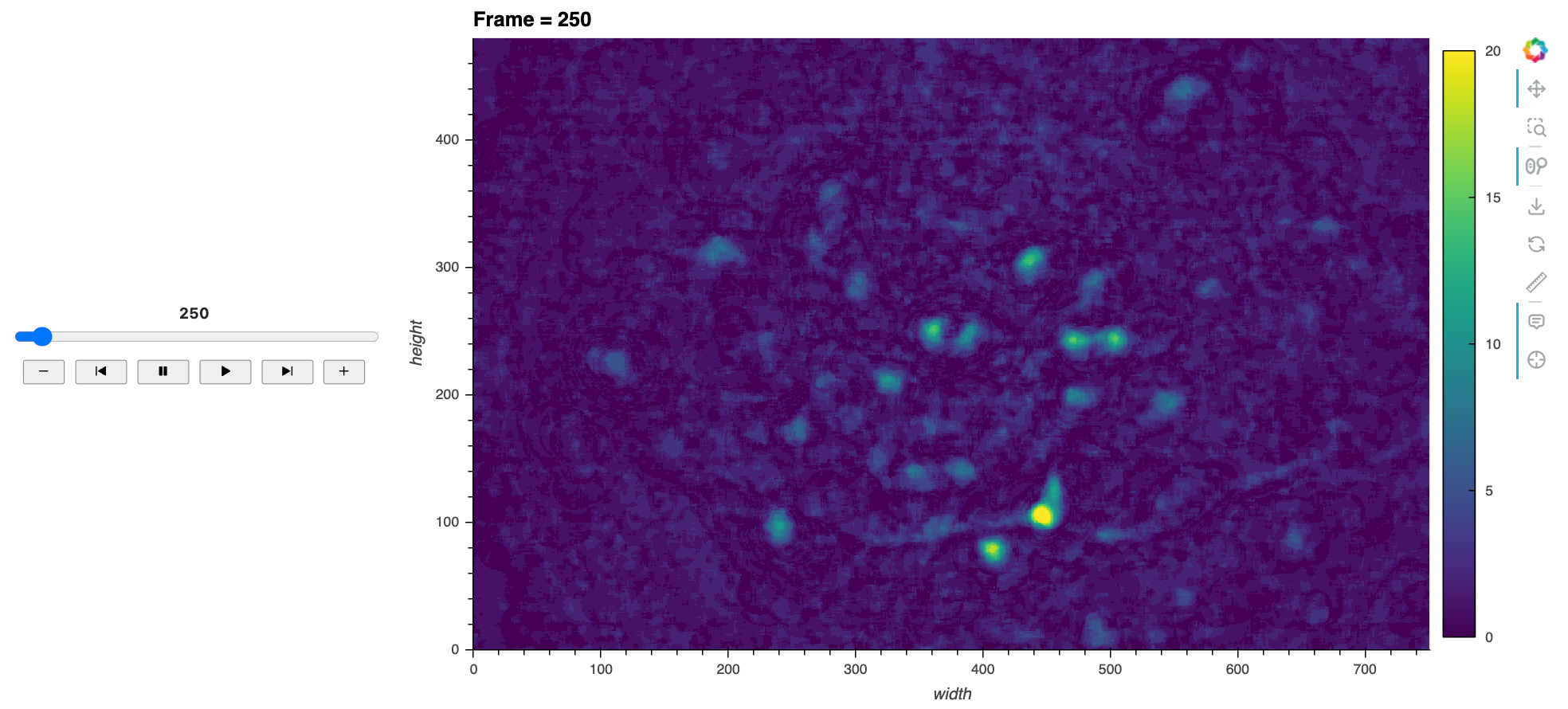
Here’s a static snapshot of the main view and frame player that we’ll make now. 👉

First, we’ll define a function to create the main image view for a given frame.

def plot_image(frame):
    return hv.Image(da.sel(frame=frame), kdims=["width", "height"]).opts(
        title=f'Frame = {frame}',
        frame_height=da.sizes['height'],
        frame_width=da.sizes['width'],
        cmap='Viridis',
        clim=(0, 20),
        colorbar=True,
        tools=['hover', 'crosshair'],
        toolbar='right',
        apply_hard_bounds=True,
        scalebar=True,
        scalebar_unit=("µm", "m"),  # Each pixel is about 1 µm in this dataset
        scalebar_opts={
            'background_fill_alpha': 0.5,
            'border_line_color': None,
            'bar_length': 0.10,
        }
    )

We’ll also create a Player widget to control frame playback.

frame_player = pn.widgets.Player(
    length=len(da.coords['frame']),
    interval=100,  # Inter-frame-interval in milliseconds
    value=20,     # Arbitrary starting frame
    show_loop_controls=False,
    align='center',
    scale_buttons=0.9,
    sizing_mode='stretch_width',
    show_value=True,
    value_align='center',
    visible_buttons=['slower', 'previous', 'pause', 'play', 'next', 'faster'],
)

We will bind (see relevant Panel docs) the main frame-wise view to the player widget. Using DynamicMap, we ensure that only the plot contents are updated, maintaining the zoom level and other plot settings across updates. Additionally, by binding to value_throttled, we update the frame only when the user releases the slider, which improves performance by avoiding unnecessary updates:

main_view = hv.DynamicMap(pn.bind(plot_image, frame_player.param.value_throttled))

Maximum Projection Overlay#

Here’s a static snapshot of the max projection with a linked opacity slider that we’ll make now. 👉

We now create a max time-projected image and a slider widget to adjust the transparency of this overlay. As before, the max projection helps in identifying areas of interest by showing the maximum value over time for each pixel. We’ll use a fast jslink approach to link to the slider to the opacity parameter of the image since this is a simple visual property update.

# Compute the maximum projection over time
max_proj_time = da.max('frame').compute().astype(np.float32)

# Create the maximum projection image
img_max_proj_time = hv.Image(
    max_proj_time, ['width', 'height'], label='Max Over Time'
).opts(
    cmap='magma',
)

# Opacity slider for the overlay
opacity_slider = pn.widgets.FloatSlider(
    start=0, end=1, step=0.1, value=0.3, name='Opacity', align='center', sizing_mode='stretch_width'
)

# Link the slider value to the overlay's alpha (opacity)
opacity_slider.jslink(img_max_proj_time, value='glyph.global_alpha')

Link(args={}, bidirectional=False, code=None, name='Link01347', properties={'value': 'glyph.global_alpha'})

Side Views#

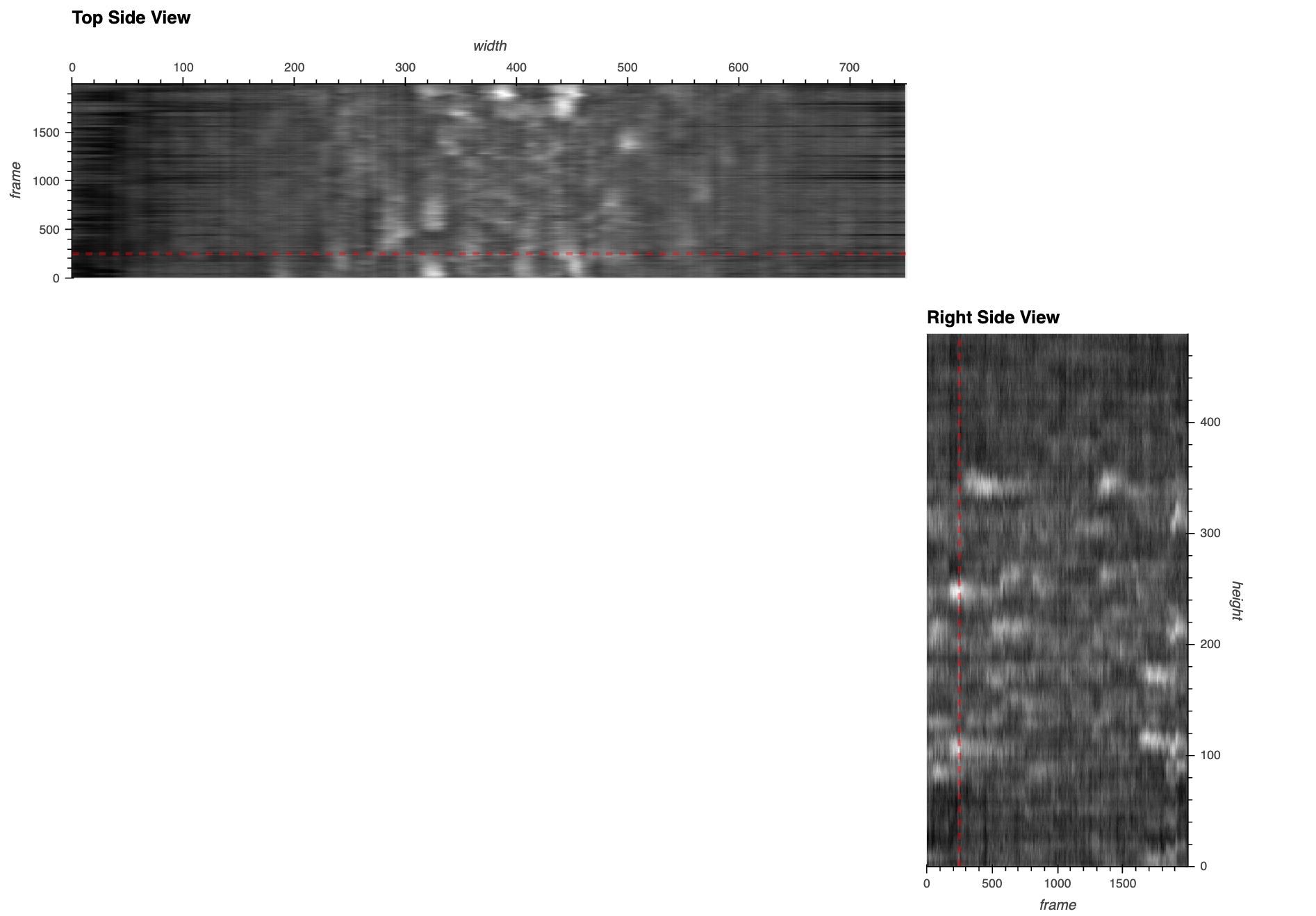
Here’s a static snapshot of the side views with a linked frame indicator lines that we’ll make now. 👉

To provide context over the time dimension, we’ll add side views showing the mean intensity over time along the height and width dimensions. The right-side view (as if looking at our 3D volume from the right side) will be a frame-by-height view, and the top-side view will be a width-by-frame view. We set axiswise=True to prevent the side views from adjusting to the range of the main view, as we want them to be stable references of the full range on their respective axes. As the dataset scales up, there’s a couple of key considerations for these views:

Using .persist() allows us to cache the results of the mean calculations, reducing recomputation and improving performance. Unlike .compute(), which loads the entire dataset into memory as a single object, .persist() retains the dataset’s chunking, making downstream operations more efficient and scalable, especially for larger datasets.

Rasterizing these views further optimizes performance by limiting the data sent to the browser. Without rasterization, the full dataset—an entire row or column of image data for each frame—must be transferred. For this small demo dataset, this means about 16 MB of data. With rasterization, only a pixel-resolution image is sent, reducing this to just 1.5 MB—a 10x improvement. The benefits grow even more as the dataset scales up, as rasterization ensures the data transferred remains proportional to the display resolution, not the dataset size. Rasterization thus maintains visual clarity while drastically reducing data transfer and ensuring efficient rendering.

# Options for the side views
side_view_opts = dict(
    cmap='greys_r',
    tools=['crosshair', 'hover'],
    axiswise=True,
    apply_hard_bounds=True,
    colorbar=False,
    toolbar=None,
)

side_view_width = 175

# Top view: mean over height
top_data = da.mean('height').persist()
top_view = rasterize(
    hv.Image(top_data, kdims=['width', 'frame']).opts(
        frame_height=side_view_width,
        frame_width=da.sizes['width'],
        title='Top Side View',
        xaxis='top',
        **side_view_opts
    )
)

# Right view: mean over width
right_data = da.mean('width').persist()
right_view = rasterize(
    hv.Image(right_data, kdims=['frame', 'height']).opts(
        frame_height=da.sizes['height'],
        title='Right Side View',
        yaxis='right',
        frame_width=side_view_width,
        **side_view_opts
    )
)

We’ll add indicators on the side views to show the current frame and the zoom range of the main view.

First, the position of these lines indicates the current frame, and updates are linked to the frame_player value. Instead of using throttled updates for the frame indicator lines, we bind directly to the unthrottled value of the frame player since this is a computationally inexpensive operation. This decision ensures that the frame indicators follow the slider in real time, providing a smooth and responsive user experience as the user scrubs through the frames.

Second, the extents of the indicator lines adjust dynamically as the user interacts with the range (zoom, pan) in the main plot. To achieve this, we use a streams.RangeXY from HoloViews, which allows us to subscribe the indicator line extents to the range of the main view plot.

def plot_hline(frame, x_range, y_range):
    if x_range is None:
        x_range = [int(da.width[0].values), int(da.width[-1].values)]
    return hv.Segments((x_range[0], frame, x_range[1], frame)).opts(axiswise=True)

def plot_vline(frame, x_range, y_range):
    if y_range is None:
        y_range = [int(da.height[0].values), int(da.height[-1].values)]
    return hv.Segments((frame, y_range[0], frame, y_range[1])).opts(axiswise=True)

line_opts = dict(color='red', line_width=3, line_alpha=0.4, line_dash='dashed')
xyrange_stream = hv.streams.RangeXY(source=main_view)
dmap_hline = hv.DynamicMap(pn.bind(plot_hline, frame_player), streams=[xyrange_stream]).opts(**line_opts, **side_view_opts)
dmap_vline = hv.DynamicMap(pn.bind(plot_vline, frame_player), streams=[xyrange_stream]).opts(**line_opts, **side_view_opts)

# Overlay the frame indicators on the side views
top_view_overlay = (top_view * dmap_hline).opts(axiswise=True)
right_view_overlay = (right_view * dmap_vline).opts(axiswise=True)

Layout#

Now we’ll assemble all components into a cohesive layout.

# Overlay the maximum projection on the main view
main_view_overlay = main_view * img_max_proj_time

# Arrange the main view and right side view horizontally
main_and_right_layout = pn.Row(main_view_overlay, right_view_overlay)

# Wrap the player and slider in collapsble Card widgets
player_layout = pn.Card(
    frame_player,
    title='Playback',
    sizing_mode='stretch_width',
    margin=(0, 0, 20, 0),
)

opacity_slider_layout = pn.Card(
    opacity_slider,
    title='Max Projection Overlay',
    sizing_mode='stretch_width',
    margin=(0, 0, 20, 0),
)

# Combine the controls
controls = pn.Column(
    player_layout,
    opacity_slider_layout,
    align='center',
    width=350,
)

# Assemble the full application layout
intermediate_app = pn.Row(
    controls,
    pn.Column(
        top_view_overlay,
        main_and_right_layout,
    )
)

# intermediate_app

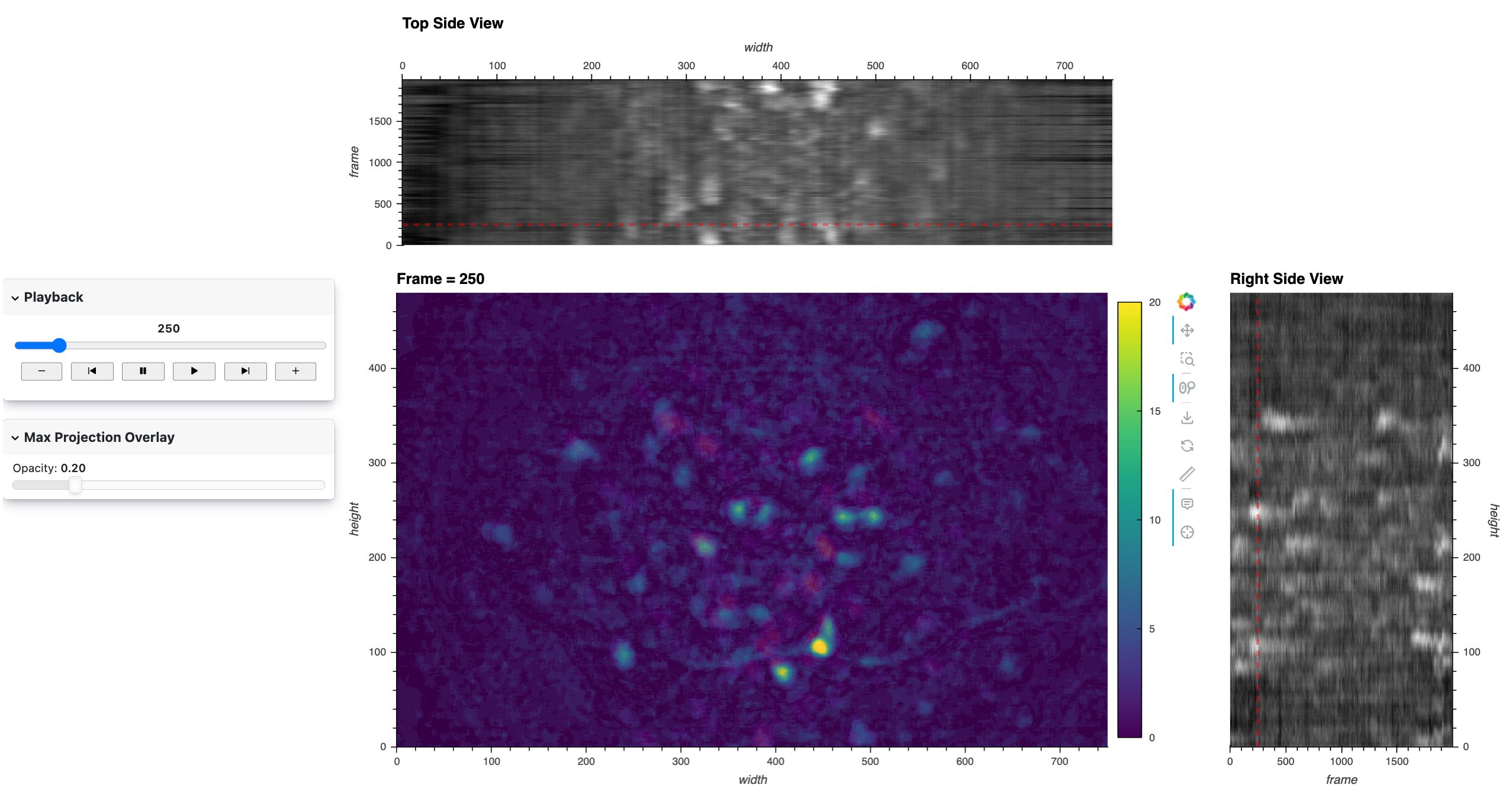
Here’s a static snapshot of what the previous cell produces - the intermediate app with side views and enhanced controls. 👉

App V3: Advanced Viewer with Annotations and Timeseries#

So far, our app allows us to navigate the image stack, but this is usually just the very start of the neuroscience investigation. From this imaging data, it’s often essential to next derive a collection of timeseries traces that reflect when individual biological neurons are more or less active, as indicated by the change in image intensity within the spatial regions occupied by each neuron.

Although there are automated approaches to aid in estimating the spatial outline of each cell, let’s work out a complementary approach of how to manually specify and log particular spatial regions of interest using HoloNote. Linked to these annotated regions of interest, we can also set up a view that populates with the mean image intensity per frame to form the estimated neural activity fluctuations over time.

Here’s a static preview of the Advanced app with the annotator controls and the linked timeseries view that we’ll now add work on. 👉

Setting Up the Annotator#

Now we’ll configure the Annotator object from HoloNote, which manages the annotations and integrates them with our plots.

In this demo, we’re using a connector to an in-memory SQLite database by specifying SQLiteDB(filename=':memory:') for temporary storage of annotations:

from holonote.annotate import Annotator
from holonote.app import PanelWidgets, AnnotatorTable
from holonote.annotate.connector import SQLiteDB

# Initialize the annotator for 'height' and 'width' dimensions
annotator = Annotator(
    {'height': float, 'width': float},
    fields=['type'],  # Additional field to categorize annotations
    groupby='type',   # Group annotations to enable color-coding and batch actions
    connector=SQLiteDB(filename=':memory:'),
)

Note on Persistent Storage: If we don’t specify a connector, HoloNote will by default create a persistent SQLite database file named ‘annotations.db’ in the current directory. You can also specify a custom filename in place of ':memory:' to store annotations persistently in a specific file, such as SQLiteDB(filename='my_annotations.db').

When working in a real workflow, you’ll likely want persistent storage to save your annotations between sessions. Be aware that if a file with the specified name already exists, HoloNote will use it, and any changes committed through the UI will modify this file. This allows you to maintain and update your annotations across different sessions, ensuring your work is saved and accessible later.

Now we can optionally choose to add colors and styling to particular annotation types. For instance, maybe we want all of ‘A’-labeled boxes to be red.

# OPTIONAL: Define colors for annotation 'types' that we might expect to make
color_dim = hv.dim('type').categorize(
    categories={
        'A': 'red',
        'B': 'orange',
        'C': 'cyan',
    },
    default='grey',
)

# Style the annotations
annotator.style.color = color_dim # apply custom colors if we made them
annotator.style.alpha = 0.3

Configuring Annotation Widgets#

To enable interaction with the annotations, we’ll create widgets that allow users to view and manage them.

# Create annotation widgets
panel_widgets = PanelWidgets(annotator)
table_widget = AnnotatorTable(
    annotator,
    tabulator_kwargs={
        'sizing_mode': 'stretch_width',
        'theme': 'midnight',
        'layout': 'fit_columns',
        'sortable': False,
        'stylesheets': [':host .tabulator {font-size: 9px;}'],
    },
)

The above code creates:

Annotation controls (PanelWidgets) for adding, editing, or deleting annotations. Since we grouped the annotations, PanelWidgets will also include a ‘Visible’ widget to toggle visibility by group.
An AnnotatorTable to display annotations in a tabular format.

We also customize the table’s appearance and functionality using tabulator_kwargs, adjusting pagination, sizing, layout, theme, style, and text alignment. Check our the Panel Tabulator docs for more options.

Timeseries of Annotated Regions#

We’ll create timeseries plots that show the mean intensity over time for each annotated region. We will connect the .on_event method of the Annotator to a plot_ts function that returns a subcoordinate timeseries plot of all the mean-aggregated spatial annotations per frame. We’ll also add a vertical line to indicate the current frame, which we’ll bind to our frame_player widget for updates.

# Options for the timeseries plot
curve_opts = dict(
    height=300,
    width=da.sizes['width'] + side_view_width + 225, # align to main_layout width
    show_legend=False,
    xlabel='Frame',
    tools=['hover'],
    line_alpha=0.5,
    framewise=True,
    axiswise=True,
)

# Options for the timeseries' frame indicator
vline_opts = dict(color='grey', line_width=4, alpha=0.5)

# Function to plot timeseries when annotations change
def plot_ts(event):
    curves = {}
    df = annotator.df
    for idx, row in df.iterrows():
        h1, h2, w1, w2 = row[['start[height]', 'end[height]', 'start[width]', 'end[width]']]
        da_sel = da.sel(height=slice(h1, h2), width=slice(w1, w2))
        mean_ts = da_sel.mean(['height', 'width'])
        group = f'G_{row["type"]}'
        label = f'L_{idx[:6]}'
        curve = hv.Curve(mean_ts, group=group, label=label)
        curve = curve.opts(
            subcoordinate_y=True,
            color=panel_widgets.colormap[row['type']],
            **curve_opts,
        )
        curves[(group, label)] = curve
    time_series.object = (vline * hv.Overlay(curves, kdims=['curve'])).opts(
        hv.opts.Curve(xlim=(frames[0], frames[-1])),
    )

# Function to create a vertical line indicating the current frame
def plot_frame_indicator_line(value):
    if value:
        return hv.VSpans((value, value)).opts(
            axiswise=True, framewise=True, **vline_opts
        )

# Get the range of frames
frames = da.coords['frame'].values

# Create a DynamicMap for the frame indicator line
vline = hv.DynamicMap(pn.bind(plot_frame_indicator_line, frame_player)).opts(
    hv.opts.VLine(**vline_opts)
)

# Initialize the timeseries pane
time_series = pn.pane.HoloViews(
    vline * hv.Curve([]).opts(
        xlim=(frames[0], frames[-1]),
        title='Create an annotation in the image',
        **curve_opts,
    )
)

# Connect the annotation events to the plotting function
annotator.on_event(plot_ts)

Defining Annotations#

Optionally, if we have some pre-existing annotations, we can add to the annotation database. If you started without any existing annotations, you can skip this step, and the Annotator will start without any entries, ready for you to add new ones interactively.

annotations_df = pd.DataFrame(
    [[430, 480, 80, 130, 'A']],
    columns=['x1', 'x2', 'y1', 'y2', 'type']
)
annotations_df

	x1	x2	y1	y2	type
0	430	480	80	130	A

annotator.define_annotations(
    annotations_df,
    width=("x1", "x2"),
    height=("y1", "y2"),
    type='type',
)

Updating the Layout#

We’ll update the application layout from the intermediate app version to include the annotator, along with the associated widgets and timeseries plot.

# Overlay the annotator on the main view
main_view_overlay_anno = (main_view_overlay * annotator).opts(axiswise=True)
# Overlay the annotator on the side views
top_view_overlay_anno = (top_view_overlay * annotator).opts(axiswise=True)
right_view_overlay_anno = (right_view_overlay * annotator).opts(axiswise=True)

# Combine annotation controls and table into a Card
annotator_widgets = pn.Card(
    pn.Column(panel_widgets, table_widget),
    title='Annotator',
    sizing_mode='stretch_width',
    margin=(0, 0, 20, 0),
    collapsed=False,
)

# Add the annotator widgets to the controls
controls.append(annotator_widgets)

# Create the main content layout
main_layout_anno = pn.Column(
    top_view_overlay_anno,
    pn.Row(main_view_overlay_anno, right_view_overlay_anno),
    time_series,
)

# Assemble the final application layout
advanced_app = pn.Row(
    controls,      # Controls on the left
    main_layout_anno,   # Main content on the right
    align='start',
)

Working with Annotations#

This video preview is a great way to see how an annotation is created with the HoloNote controls.

How to add new annotations:

Ensure that ‘Box select (x-axis)’ is selected in the Bokeh Toolbar on the right of the main frame plot.
Ensure that the ‘+’ button is selected in the Annotation widgets on the very left.
Select a spatial range by clicking and dragging on the main frame plot.
Enter the name of the group that you want the annotation to be added to in the ‘type’ text box.
Click the check (✔️) to apply the annotation.
Optionally, if you are using a persistent file on disk for the annotations and are ready to commit, hit the triangle button in the Annotation widgets to commit changes to the file.

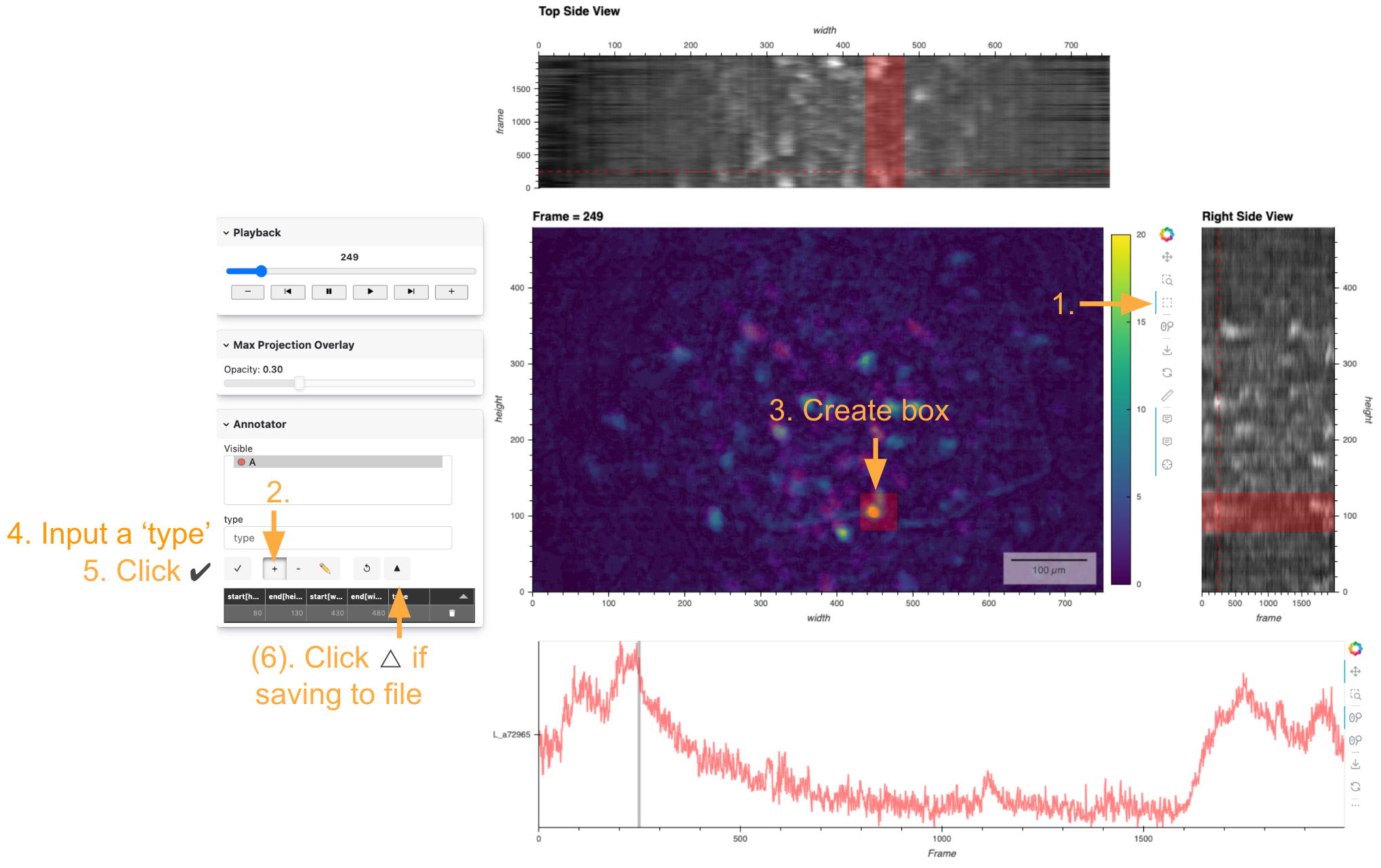
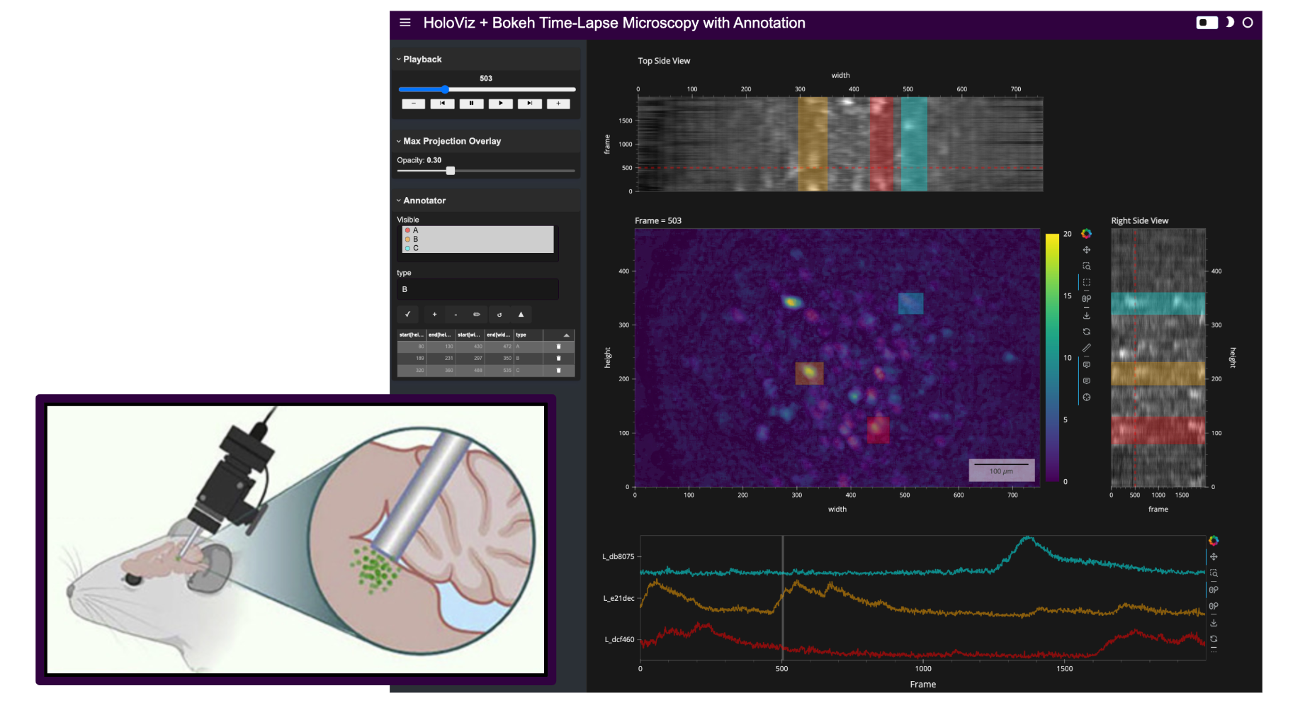
Here’s a static snapshot of what the advanced app looks like in the notebook, after creating a box in the main view and assigning it a type in the annotation widget. 👉

advanced_app

Standalone App Extension#

HoloViz Panel allows for the deployment of this complex visualization as a standalone, template-styled, interactive web application (outside of a Jupyter Notebook). Read more about Panel here.

We’ll add our plots to the main area of a Panel Template component and the widget-controls to the sidebar. Finally, we’ll set the entire component to be servable.

To launch the standalone app, activate the same conda environment and run panel serve <path-to-this-file> --show in the command line to open the application in a browser window (tip: use the --dev flag to auto update the app when the file changes).

Warning

It is not recommended to have both a notebook version of the app and the served version of the same application running simultaneously. Prior to serving the standalone application, clear the notebook output, restart the notebook kernel, and save the unexecuted notebook file.

servable_app = pn.template.FastListTemplate(
    sidebar = controls,
    title = "HoloViz + Bokeh Time-Lapse Microscopy with Annotation",
    main = main_layout_anno,
    main_layout=None,
    sidebar_width=350,
    theme="dark",
    accent="#30023f"
).servable()

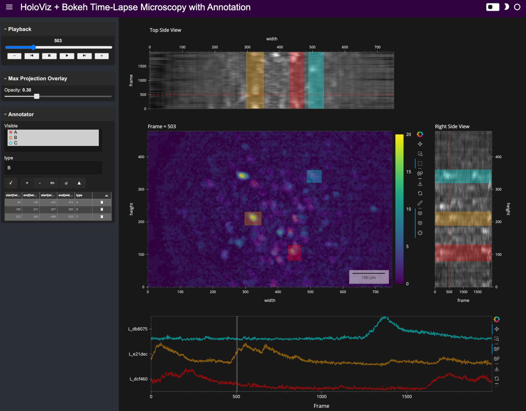
Here’s a static snapshot of what the standalone app looks like in a browser window. 👉

Copyable V3 App Code#

Expand to reveal

from pathlib import Path
import numpy as np
import pandas as pd
import xarray as xr
import holoviews as hv
from holoviews.operation.datashader import rasterize
import panel as pn
import fsspec
from holonote.annotate import Annotator
from holonote.app import PanelWidgets, AnnotatorTable
from holonote.annotate.connector import SQLiteDB

pn.extension('tabulator')
hv.extension('bokeh')

# Load Data
DATA_URL = 'https://datasets.holoviz.org/miniscope/v1/real_miniscope_uint8.zarr/'
DATA_DIR = Path('./data')
DATA_FILENAME = Path(DATA_URL).name
DATA_PATH = DATA_DIR / DATA_FILENAME

DATA_DIR.mkdir(parents=True, exist_ok=True)
if not DATA_PATH.exists():
    ds_remote = xr.open_dataset(fsspec.get_mapper(DATA_URL), engine='zarr', chunks={})
    ds_remote.to_zarr(str(DATA_PATH))

ds = xr.open_dataset(
    DATA_PATH,
    engine='zarr',
    chunks={'frame': 400, 'height': -1, 'width': -1}
)
da = ds['varr_ref']

# Player Widget
frame_player = pn.widgets.Player(
    length=len(da.coords['frame']),
    interval=100,
    value=20,
    show_loop_controls=False,
    align='center',
    scale_buttons=0.9,
    sizing_mode='stretch_width',
    show_value=True,
    value_align='center',
    visible_buttons=['slower', 'previous', 'pause', 'play', 'next', 'faster'],
)

# Main Image View Function
def plot_image(frame):
    return hv.Image(da.sel(frame=frame), kdims=["width", "height"]).opts(
        title=f'Frame = {frame}',
        frame_height=da.sizes['height'],
        frame_width=da.sizes['width'],
        cmap='Viridis',
        clim=(0, 20),
        colorbar=True,
        tools=['hover', 'crosshair'],
        toolbar='right',
        apply_hard_bounds=True,
        scalebar=True,
        scalebar_unit=("µm", "m"),  # Each pixel is about 1 µm in this dataset
        scalebar_opts={
            'background_fill_alpha': 0.5,
            'border_line_color': None,
            'bar_length': 0.10,
        },
    )

# Bind the Main View to the Frame Player
main_view = hv.DynamicMap(pn.bind(plot_image, frame_player.param.value_throttled))

# Maximum Projection Overlay
max_proj_time = da.max('frame').compute().astype(np.float32)
img_max_proj_time = hv.Image(
    max_proj_time, ['width', 'height'], label='Max Over Time'
).opts(
    cmap='magma',
)
opacity_slider = pn.widgets.FloatSlider(
    start=0, end=1, step=0.1, value=0.3, name='Opacity', align='center', sizing_mode='stretch_width'
)
opacity_slider.jslink(img_max_proj_time, value='glyph.global_alpha')

# Annotator Setup
annotator = Annotator(
    {'height': float, 'width': float},
    fields=['type'],  # Additional field to categorize annotations
    groupby='type',   # Group annotations to enable color-coding and batch actions
    connector=SQLiteDB(filename=':memory:'),
)

# Define Colors for Annotation Types
color_dim = hv.dim('type').categorize(
    categories={
        'A': 'red',
        'B': 'orange',
        'C': 'cyan',
    },
    default='grey',
)
annotator.style.color = color_dim
annotator.style.alpha = 0.3

# Annotation Widgets
panel_widgets = PanelWidgets(annotator)
table_widget = AnnotatorTable(
    annotator,
    tabulator_kwargs={
        'sizing_mode': 'stretch_width',
        'theme': 'midnight',
        'layout': 'fit_columns',
        'sortable': False,
        'stylesheets': [':host .tabulator {font-size: 9px;}'],
    },
)

# Timeseries Plot
curve_opts = dict(
    height=300,
    width=da.sizes['width'] + 175 + 225,  # Adjust width to align with main layout
    show_legend=False,
    xlabel='Frame',
    tools=['hover'],
    line_alpha=0.5,
    framewise=True,
    axiswise=True,
)

vline_opts = dict(color='grey', line_width=4, alpha=0.5)

def plot_ts(event):
    curves = {}
    df = annotator.df
    for idx, row in df.iterrows():
        h1, h2 = row[['start[height]', 'end[height]']]
        w1, w2 = row[['start[width]', 'end[width]']]
        da_sel = da.sel(height=slice(h1, h2), width=slice(w1, w2))
        mean_ts = da_sel.mean(['height', 'width'])
        group = f'G_{row["type"]}'
        label = f'L_{idx[:6]}'
        curve = hv.Curve(mean_ts, group=group, label=label)
        curve = curve.opts(
            subcoordinate_y=True,
            color=panel_widgets.colormap.get(row['type'], 'grey'),
            **curve_opts,
        )
        curves[(group, label)] = curve
    time_series.object = (vline * hv.Overlay(curves)).opts(
        hv.opts.Curve(xlim=(frames[0], frames[-1]))
    )

def plot_frame_indicator_line(value):
    if value is not None:
        return hv.VSpan(value, value + 1).opts(
            axiswise=True, framewise=True, **vline_opts
        )

frames = da.coords['frame'].values
vline = hv.DynamicMap(pn.bind(plot_frame_indicator_line, frame_player.param.value)).opts(**vline_opts)
time_series = pn.pane.HoloViews(
    vline * hv.Curve([]).opts(
        xlim=(frames[0], frames[-1]),
        title='Create an annotation in the image',
        **curve_opts,
    )
)
annotator.on_event(plot_ts)

# Side Views
side_view_opts = dict(
    cmap='greys_r',
    tools=['crosshair', 'hover'],
    axiswise=True,
    apply_hard_bounds=True,
    colorbar=False,
    toolbar=None,
)

side_view_width = 175

# Top View: Mean over height
top_data = da.mean('height').persist()
top_view = rasterize(
    hv.Image(top_data, kdims=['width', 'frame']).opts(
        frame_height=side_view_width,
        frame_width=da.sizes['width'],
        title='Top Side View',
        xaxis='top',
        **side_view_opts
    )
)

# Right View: Mean over width
right_data = da.mean('width').persist()
right_view = rasterize(
    hv.Image(right_data, kdims=['frame', 'height']).opts(
        frame_height=da.sizes['height'],
        frame_width=side_view_width,
        title='Right Side View',
        yaxis='right',
        **side_view_opts
    )
)

# Indicator Lines on Side Views
def plot_hline(frame, x_range, y_range):
    if x_range is None:
        x_range = [int(da.width[0].values), int(da.width[-1].values)]
    return hv.Segments((x_range[0], frame, x_range[1], frame)).opts(axiswise=True)

def plot_vline(frame, x_range, y_range):
    if y_range is None:
        y_range = [int(da.height[0].values), int(da.height[-1].values)]
    return hv.Segments((frame, y_range[0], frame, y_range[1])).opts(axiswise=True)

line_opts = dict(color='red', line_width=3, line_alpha=0.4, line_dash='dashed')
xyrange_stream = hv.streams.RangeXY(source=main_view)
dmap_hline = hv.DynamicMap(
    pn.bind(plot_hline, frame_player.param.value, xyrange_stream.param.x_range, xyrange_stream.param.y_range)
).opts(**line_opts, **side_view_opts)
dmap_vline = hv.DynamicMap(
    pn.bind(plot_vline, frame_player.param.value, xyrange_stream.param.x_range, xyrange_stream.param.y_range)
).opts(**line_opts, **side_view_opts)

# Overlay the frame indicators on the side views
top_view_overlay = (top_view * dmap_hline).opts(axiswise=True)
right_view_overlay = (right_view * dmap_vline).opts(axiswise=True)

# Layout

# Overlay the maximum projection and annotator on the main view
main_view_overlay_anno = (main_view * img_max_proj_time * annotator).opts(axiswise=True)

# Overlay the annotator on the side views
top_view_overlay_anno = (top_view_overlay * annotator).opts(axiswise=True)
right_view_overlay_anno = (right_view_overlay * annotator).opts(axiswise=True)

# Wrap the player and slider in collapsible Card widgets
player_layout = pn.Card(
    frame_player,
    title='Playback',
    sizing_mode='stretch_width',
    margin=(0, 0, 20, 0),
)

opacity_slider_layout = pn.Card(
    opacity_slider,
    title='Max Projection Overlay',
    sizing_mode='stretch_width',
    margin=(0, 0, 20, 0),
)

# Combine annotation controls and table into a Card
annotator_widgets = pn.Card(
    pn.Column(panel_widgets, table_widget),
    title='Annotator',
    sizing_mode='stretch_width',
    margin=(0, 0, 20, 0),
    collapsed=False,
)

# Combine the controls
controls = pn.Column(
    player_layout,
    opacity_slider_layout,
    annotator_widgets,
    align='center',
    width=350,
)

# Create the main content layout
main_layout_anno = pn.Column(
    top_view_overlay_anno,
    pn.Row(main_view_overlay_anno, right_view_overlay_anno),
    time_series,
)

# Assemble the final application layout for use in a notebook
advanced_app = pn.Row(
    controls,      # Controls on the left
    main_layout_anno,   # Main content on the right
    align='start',
)

# Create the servable standalone app
servable_app = pn.template.FastListTemplate(
    sidebar=controls,
    title="HoloViz + Bokeh Time-Lapse Microscopy with Annotation",
    main=main_layout_anno,
    main_layout=None,
    sidebar_width=350,
    theme="dark",
    accent="#30023f"
).servable()

advanced_app

Next Steps#

Experiment with your own datasets, extending the applications with additional features as needed.

Resources#

What?	Why?
Minian Repository	Analysis pipeline and visualization tool for Miniscope data
Miniscope Wiki	Further context for the demo application
HoloNote	HoloNote package for annotation capabilities in HoloViz applications

This web page was generated from a Jupyter notebook and not all interactivity will work on this website.